Beware: lowering GC time may not lead to better application performance

One of the most established approaches to improve Java application performance is to tune JVM options, in particular Garbage Collector (GC) parameters. 

Indeed, the main task of garbage collection is to free memory up which requires stopping the application threads during the stop-the-world (STW) pause, after which application threads are resumed in their execution when the garbage collection has completed. The STW interval is measured by the GC pause metric.

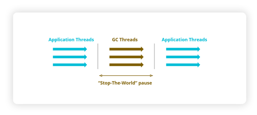
The percentage of time spent in performing garbage collection is called GC time or GC overhead.

The conventional wisdom of GC performance is that you must always try to lower GC time as much as possible. This seems to make sense as by decreasing GC time, we get higher throughput meaning that the application threads can run for longer without interruption. However, when running actual optimization studies it results that things can be very different than expected, as we will see in the following.

GC Time and application performance: what happens behind the scenes

The following chart, taken from the official Oracle documentation, shows the impact of GC time percentage on application throughput and also scalability.

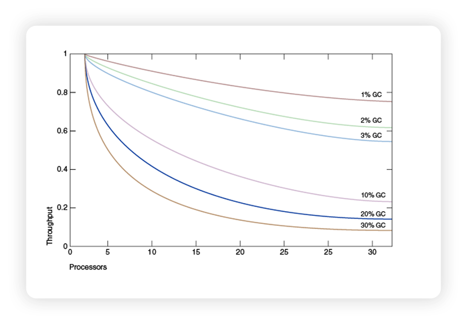
These curves basically follow the well-known Amdhal’s law, which states that the speedup on a parallel program is limited by the sequential part. In Java, the sequential part is actually the GC pause, the rest is the parallel processing.

Looking at this chart, it is easy to understand why the general goal of improving Java application throughput via JVM tuning is stated as the following “golden” rule: “keep the overhead of doing garbage collection as low as possible” (as stated in the Oracle documentation).

This performance rule is so ingrained in our industry practices that, in addition to representing the main best practice for JVM tuning activities, it is also hardcoded by many APM tools when recommending how to tune JVM.

However, the GC overhead is far from being the only factor driving application performance, as we are going to discuss next. And more importantly, that by only focusing on reducing the GC overhead you actually may end up slowing your application down – a very counterintuitive fact!

Looking deeper into GC behaviour

In order to see how much the GC behaviour can be counterintuitive, we can use Renaissance, a popular open-source Java benchmarking suite (renaissance.dev) that includes a Spark-based application running on OpenJDK 11, and study how application execution time varies when the JVM and GC parameters are tuned.

To simplify this task we leveraged Akamas, our AI-powered optimization solution. Akamas allows the benchmark to be launched with different JVM configurations and automatically find an optimal configuration driven by a custom goal such as minimizing execution time. This allowed us to perform 80 experiments executed in just about 20 hours in an unattended way.

The following chart shows the results of this study, where each dot represents a benchmark execution with a specific set of JVM options: the yellow dot represents the JVM with default settings (baseline configuration) and the red dot the optimal configuration.

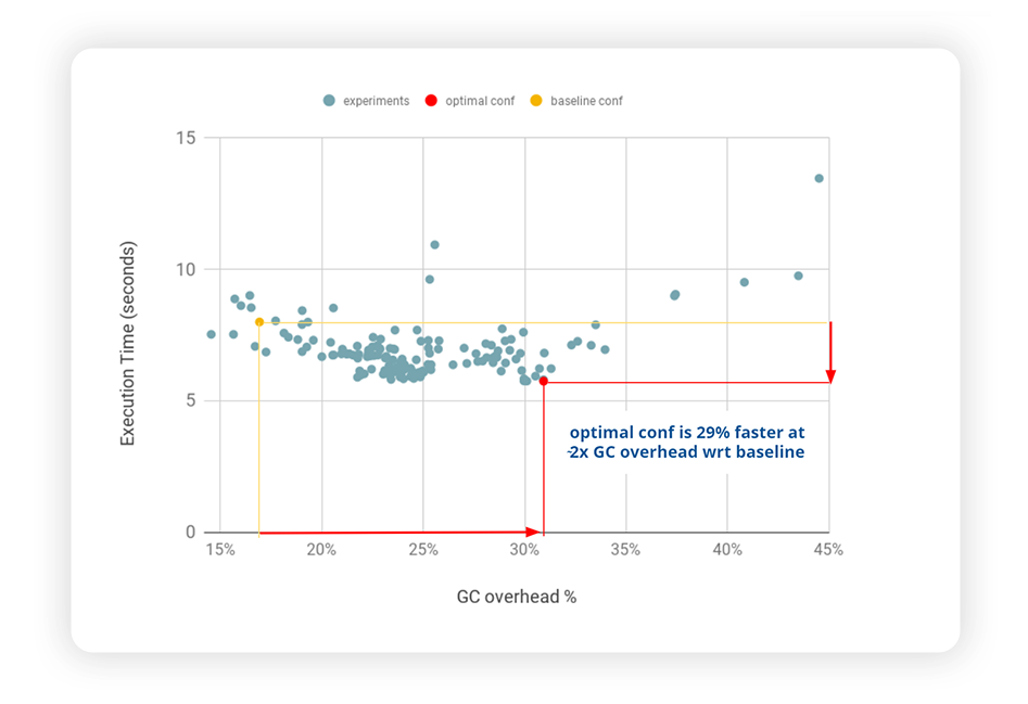
This chart reveals a couple of quite interesting findings:

• The best configuration makes the application 29% faster than the baseline – not a small improvement, which was achieved by simply reconfiguring the JVM
• The best configuration corresponds to a higher GC overhead! – by almost a factor of 2x – this is very counterintuitive and not aligned to the golden rule!!

It is also interesting to comment on the shape of this curve. We might have expected a somewhat linear relationship between overhead and execution time – the higher the GC overhead, the higher the execution time. Instead, the optimal minimum execution times are achieved at around 30% GC overhead values.

It is also worth noting that the baseline shows a GC overhead at 15%, which is typically considered quite high. As a matter of fact, some APM tools warn about a “high overhead” already at 15%. And here, the very surprising finding is that a configuration with higher GC overhead (29%) makes the application go faster.

All these findings raise the question: how on earth can an application run faster when GC is leaving less time for the application threads to run? We had to go deeper – at the OS level where the JVM threads get scheduled – in order to find the answer.

What happens behind the scenes

In order to better understand the dynamics of JVM performance, we analyzed how the application and GC threads are managed by the Linux CPU scheduler on the actual processors.

There are several tracing tools that can be used for this purpose. For example Linux perf, the main low-level performance analysis tool for the Linux OS, or ftrace, a facility built into the Linux kernel that is able to trace scheduling events. We decided to use Perfetto, a browser-based tracing tool built by Google, which is probably better known as a tool used by Android developers to diagnose mobile app performance issues, but which works on standard Linux OS distributions and also provides a nice visualization.

The following chart shows the different JVM threads (one for each row) as they are scheduled on the CPUs: application threads are listed at the top (Executor tasks), while the GC threads are displayed at the bottom. The latter are the JVM threads that actually perform the GC work. For each thread, the bar shows when a thread is actually running: dark green when the thread is running on the CPU and light green when it is waiting to access the CPU.

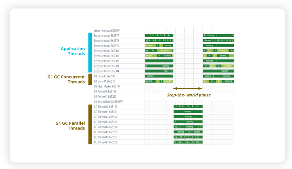
Second, you can notice that there are also some GC threads that are executed concurrently with the application threads. They are called “G1 Conc” and this is a design feature of the OpenJDK 11 G1 Garbage Collector which uses background threads to perform part of the garbage collection process, introduced with the goal of reducing the STW pause. 

Therein we can find the answer for the surprising behaviour of a higher GC overhead corresponding to a faster application. Indeed, the G1 GC concurrent threads are “competing” with the application threads for CPU resources. Since these GC threads work concurrently with the application threads, they are not counted in the GC overhead, which trumps the “golden” rule.

Therefore, when tuning the JVM if you just follow the golden rule of reducing the GC overhead, as you cannot be sure that this will improve your application performance! Actually, you may cause more harm than good as you might be asking the Garbage Collector to do more concurrent work, which may keep the application threads waiting, thus causing the application to be slowed down.

Conclusions

The key takeaway is that while GC time remains an important metric to observe, as performance engineers we need to keep in mind that the simple “golden” rule of always trying to reduce GC overhead does not always work. This rule relies on a simplistic model of what actually happens at the JVM level, which does not hold true anymore in modern systems, where the JVM and the underlying system interact in complex and sometimes unpredictable ways – which has relevant effects on the end-to-end application performance.

This is just an instance of a general situation in today’s practice of performance tuning. These days, the complexity of applications (whether monolithic or microservice-based) and infrastructures (whether on premise, cloud or hybrid) makes it very difficult to approach performance tuning by relying on pre-defined rules and vendor best practices. 

Akamas provides Performance Engineers with the ability to optimize application performance by smartly exploring thousands of configurations, without relying on predefined rules and human knowledge. Akamas specialized AI techniques always finds the optimal configuration with respect to your custom goals (e.g. performance and cost tradeoffs) and constraints (e.g. SLOs), in just a few hours.

In the following blog entries we will continue to debunk other JVM performance tuning myths and advocate for a new approach to performance optimization. Stay tuned!